 | ( 2 ) |
Pierre C. J. Hoogenboom and Cor Kasbergen
Department of Civil Engineering, Delft University of Technology
Delft, The Netherlands
It becomes gradually accepted that safety factors and design values in codes of practice should be calculated from sensitivity factors and safety indices. Currently this is not always the case and a continuing effort is going on to make codes consistent with this basic philosophy. A clear way to show the discrepancy between theory and codes is to compute the safety indices directly from a set of safety factors. The paper presents a simple method for this and demonstrates it on a number of examples showing that structural safety realized in practice varies considerably.
The theory of structural reliability is well developed now, however, its applications are for a large part limited to computations that support the development of codes of practice. The research presented in this paper attempts to make part of the reliability theory accessible for practical structural design. In Section 2 of the paper the classical way to derive safety factors is summarized. However, it is no secret that to date this theory is still not consistently applied: Safety factors in codes of practice are often rather a political compromise than accurately derived from reliability requirements.
Therefore, accepting the safety factors, in the subsequent Sections of the paper a method is proposed to compute structural reliability directly from a set of load combinations. The question we address is: What will be the reliability of a structure when a specific set of load combinations is used in its design. So, we do not want to design the structure first and find out after full probabilistic analysis that it is not safe enough (or perhaps too safe) for the obvious reason that than it is too late to make substantial changes.
Structures are designed to resist sets of load combinations that are associated with a limit state. Each load combination contains load cases and safety factors. A general example of a load combination is
| R gR > W gW & P gP & S gS | ( 1 ) |
It states that the strength has to be larger than the load. In the equation W, P, S are load cases and gW, gP, gS are safety factors. Examples of load cases are wind, pre-stressing and material shrinkage. R is a strength parameter like the concrete compression strength and gR is a safety factor related to this strength. In North American codes gR is denoted as f and in European codes it is denoted as 1/gm. In this paper we use gR to obtain a simple formulation.
The safety factors of a load combination can be calculated easily according to the theory of probability (Cornell 1969). If we restrict ourselves to normally distributed variables the formula is
In this, b is the target reliability index, which depends on the limit state that is associated with the load combinations. V is the variation coefficient of either a load case or a strength parameter, m is its average and k is the characteristic value of a load case that will be used in the design. The factors a are sensitivity factors which are defined with the standard deviations of the load cases and the limit state function. Since the limit state function is not known in design the sensitivity factors are approximated using the property that the length should be equal to 1.
 | ( 3 ) |
In this, k is the number of load cases (basic variables). In order to be at the safe side the approximated sensitivity factors should have a length somewhat more than 1 for each load combination (Vrouwenvelder 1996).
Load cases often vary in time which can be taken into account with Turkstraĺs rule. In Turkstraĺs rule in turn one of the load cases has the extreme distribution of its stochastic process while the other load cases have an instantaneous distribution. (see Appendix).
In the first example below it is demonstrated that the safety factors of the load combinations of a limit state can be calculated conveniently.
If the safety factors are known, the safety index can be computed as shown in this Section. This procedure is more elaborate than the calculations in the previous Section but it can be processed conveniently by software.
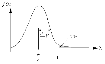
We start with the load cases. Each load case can be multiplied with a stochastic load factor l . So, when this load factor equals 1 the characteristic load is applied at the structure. When it equals g the design load is at the structure (see figure 1). A similar stochastic factor l can be defined for each strength parameter.
|
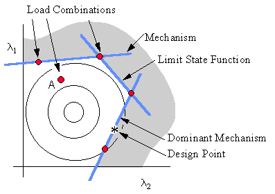
All factors l create a space of basic variables. A load combination is a point in this space. A convex envelope can be constructed around these points. In figure 2, two dimensions of the space of basic variables are drawn. The dots in the figure are load combinations. The lines trough the dots are linear mechanisms which create a target limit state function. In the example of this figure, one of the load combinations with label A is not on the convex limit state function. Apparently, this combination is not relevant for the structural safety.
The limit state function of a structural design that stands up to all load combinations will be just outside the envelope. So, the envelope can be used to compute the safety of the structure. We will refer to this envelope of the load combinations as the target limit state function.
|
In case of structural elements like beams or columns the limit state function will in general not closely match the target limit state function. However, when a whole structure is considered the limit state function consists of many individual mechanisms. This limit state function is expected to be close to the target limit state function. This is confirmed by an observation in structural design: In case of a simply supported beam often one load combination is governing for dimensioning while in case of a large structure each load combination is important since each can be governing somewhere in the structure.
When the target limit state function and the stochastic properties of the load cases are known, the failure probability can be computed with standard reliability procedures. For this project we selected Turkstraĺs rule in combination with Ditlevsenĺs narrow bounds as explained below (Turkstra 1972) (Ditlevsen 1979).
A target limit state function consists of a large number of mechanisms. Each mechanism is a linear hyperplane in the space of basic variables l. The safety margin G of a mechanism is formulated such that when the structure is about to fail the safety margin is nil and when the safety margin is negative the structure has failed.
| G = lT n | ( 4 ) |
In this, n is the normal vector of the hyperplane. When the structure is safe the safety margin is positive, say 1.
| 1 = pT n | ( 5 ) |
In this, p is a vector to the point of average values in hyperspace. A selected load combination g should be at the hyperplane. So,
| 0 = giT n . | ( 6 ) |
Suppose we have k load cases than k-1 load combinations are required to create a unique hyperplane. Often it occurs that less independent load combinations are available. In that case the normal vector n of the hyperplane is chosen to be in the direction of the point of average values. So, n is a linear combination of the vectors gi in the hyperplane and p outside this plane.
In this, j is the number of load combinations that are used to compute the hyperplane and hi is a combination factor.
The left hand part of figure 3 shows the hyperplane in case k-1 load combinations are available (k is the number of basic variables). The right hand part of the figure illustrates the hyperplane when less combinations are used.
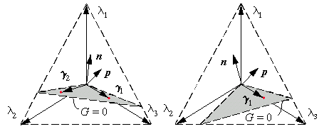
Figure 3: Mechanisms defined as planes in a space of three basic variables
Formula (5), (6) and (7) provide 1+j+k equations from which the same number of unknown can be solved. The unknown are h1 to hj+1 and n1 to nk . A convenient algorithm assembles the vectors gi and p in a matrix L. Thus, equation (7) becomes
and equation (5) and (6) can be written as
| b = LT n . | ( 9 ) |
In which b is a column vector with the elements [0, 0, ... 0, 1].
Substituting (8) in (9) we get
| b = LT L h | ( 10 ) |
from which h can be solved with a standard solver for a linear sets of equations. Finally, substituting h in equation (8) we can compute n with which a hyperplane is determined.
The algorithm we employed for computation of the safety index and failure probability consists of three parts:
1 Limit State Function
The target limit state function is a convex envelope of the load combinations in the space of basic variables (see figure 2). It is determined by generating all combinations of load combinations and creating for each combination a hyperplane. If no load combination is outside this plane it is selected as mechanism of the target limit state function.
2 Safety Indices
Turkstraĺs rule was adopted to approximate the extreme value in a reference period (Turkstra 1972). So, in turn one of the load cases has the extreme distribution of its stochastic process while the other load cases have an instantaneous distributions of their stochastic processes. For example,  in which
  and
and  are stochastic processes. The probability that the mechanism G = 0 is crossed in a reference period is approximated as the largest probability of
 | ( 11 ) |
In this li1 is a stochastic variable. the superscript i refers to an instantaneous distribution and the superscript e to the extreme distribution in a certain reference period (see Appendix).
The safety indices b and correlation coefficients are computed for each mechanism and each Turkstra combination.
This safety index, proposed by Basler and Cornell (Cornell 1969), gives the same result as the Hasofer-Lind safety index (Hasofer 1974) due to the simple definition of the safety margin G. Of course, the smallest of all safety indices is governing.
3 Failure Probability
The upper and lower bounds of the failure probability are computed according to Ditlevsen (Ditlevsen 1979) assuming normally distributed load factors.
Next to the safety index and the failure probability the algorithm provides additional information. For example the dominant mechanism, the dominant load combination and the dominant load case. Also the load combinations are identified that do not participate in the limit state function. The design point can be computed easily as the point at the limit state function with the highest probability density.
In this Section the algorithm explained above is applied to three situations.
Validation
In this example, first the safety factors are calculated based on a target safety index and subsequently the inverse procedure is used to compute the safety index from the safety factors. We choose a target safety index of 3.5 which is often used for ultimate limit states. The used sensitivity factors are shown in table 1.
|
|
The statistical properties of the load factors and strength factors are presented in table 2. In the table mii/ki is the mean of the instantaneous distribution of a load factor or strength. Vii is the instantaneous variation coefficient of a factor. mei/ki is the mean of the extreme distribution while Vie is the variation coefficient of the extreme distribution. The factor l1 represents wind load at the Dutch coast while factor l2 is the load at office floors. The third factor is the strength of steel. The reference period (design life) of the extreme distributions is 50 years.
This data was used to calculate safety factors using equation (2). The result is displayed in table 3. The load distributions were in turn extreme so that 8 load combinations appear. The load combinations and limit state function are drawn in figure 4.
|
Figure 4: The space of basic load variables of the first example (l3 = 1.05). |
Using the algorithm described before a safety index of 3.48 is computed. This is slightly less then the target safety index of 3.50 initially used for calculation of the safety factors.
Continuous Deep BeamA concrete deep beam continuing over four supports was designed according to the Dutch code (NEN 1991). Figure 5 gives an impression of the structure. The deep beam supports a three story steel frame of an industry building. It is emphasized that the exact geometry of the design is irrelevant for the example.
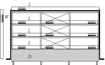
Figure 5: A continuous deep beam supporting a steel frame
The following load combinations were used in its design.
In this are fc the concrete compression strength, D the dead load including the walls weight, L the live load and W the wind load. Because the structure is symmetrical only wind from one direction is considered. The following statistical data was found in literature for the Dutch situation (see table 4) (Vrouwenvelder 1997).
|
m i / k |
V i |
m e / k |
V e |
|
|
fc |
1.50 |
0.15 |
||
|
D |
1.05 |
0.05 |
||
|
L |
0.30 |
0.40 |
1.00 |
0.40 |
|
W |
0.15 |
1.10 |
1.30 |
0.21 |
The program computes the safety index b = 2.5 and finds that the wind load is dominant for the safety. The safety is not sufficient since the Dutch code of practice requires a minimum safety index of bo = 2.6 in case the structure fails due to wind (NEN 1990).
Offshore Structure
As a final example we compute the safety of a reinforced concrete offshore structure designed with the Norske Veritas code. This codes uses the following load combinations for design of offshore structures (CIRIA 1976).
The used symbols are clarified in table 5. In this example we selected the environmental conditions as shown in table 5 that could represent a location at the north see. So, not a specific structure is checked and neither the general correctness of the Norske Veritas code is considered.
|
m i / k |
V i |
m e / k |
V e |
||
|
fy |
Steel Yield Strength |
1.30 |
0.08 |
||
|
fc |
Concrete Crushing Strength |
1.30 |
0.15 |
||
|
D |
Dead Load |
1.05 |
0.07 |
||
|
Q |
Live Load (Imposed Load) |
0.30 |
0.40 |
1.00 |
0.40 |
|
W |
Wind Load |
0.15 |
1.10 |
1.20 |
0.20 |
|
P |
Hydrostatic Pressure |
0.60 |
0.40 |
1.20 |
0.40 |
With this data the program computes a safety index b = 3.0. The dominant mechanism is
which includes the load combinations 2, 3 and 4. The dominant load case is the wind load W since the governing safety index is computed when the wind load is extreme. Note that in load combination 2 the safety factor of the dead load D is small because the dead load might be contributing to the strength of the structure. So, in the dominant mechanism, D is a strength variable instead of a load case.
The algorithm runs on a normal modern personal computer and takes less than a second of computation time for a normal number of load cases. A simple Windows interface was build to make the theory accessible to others. The main window of the program is shown in figure 6. The software can be down loaded from the WWW at:
The algorithm needs at least one strength variable and at least one load case because of the piece wise linear target limit state function. Of course in practice this condition is always met.
Two improvements of the proposed algorithm are being investigated. First, the software can be expanded such that other than normal distributions can be processed. Second, Turkstraĺs rule can be replaced with the more accurate Ferry-Borges Castanheta rule (Ferry-Borges et al. 1971). On top of this it is planned to include a data base with load data in future versions of the software.
It has to be mentioned that using other safety factors than the ones stated in codes of practice is often still not allowed. Only the national codes of some small countries allow probabilistic computations to proof the validity of a design. For example Dutch code (NEN 1991).
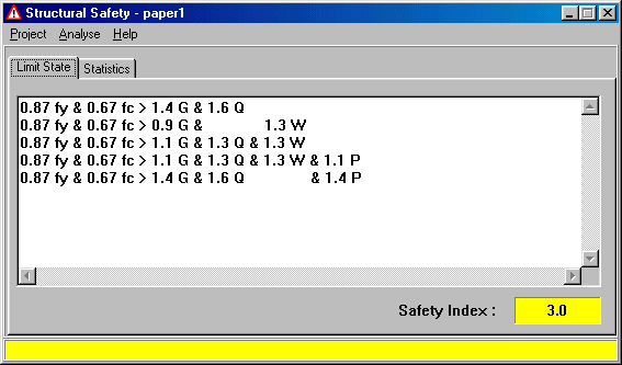
Figure 6: A windows program for computation of the safety index
The safety index of a limit state and its failure probability can be computed directly from safety factors and load combinations. Modern PC software can make this information conveniently available to every structural designer. With this software, safety factors can be checked to guaranty sufficient reliability and they can be improved for special projects.
We gratefully mention the discussions with Prof. A. Vrouwenvelder and Prof. J. Schneider during the development of the algorithm. Also we like to acknowledge the valuable comments of Dr. H. Karadeniz in preparing this paper.
Turkstraĺs rule can be formulated as follows (Turkstra 1972). Consider k processes x which vary in time t.
The time is restricted to a reference period T. So,
Consider a combined effect G of the processes x
So, G is a function of t too. The probability that G out-crosses a limit a in the reference period is denoted as
Turkstraĺs rule approximates this probability as the largest of k probabilities
In this formulation Gi is
and

In this is xj(t*) a value of the process at any time t* and max{xj(t)} is the largest value of the process in reference period T.
In case G is a linear function its mean mG and standard deviation sG can be easily computed with the mean and standard deviation of xj(t*) and max{xj(t)} as shown in equation (12).